

How Could I Visualize The Data From Mothur
Overview
In this tutorial we will perform an analysis based on the Standard Operating Process (SOP) for MiSeq data, developed by the Schloss lab, the creators of the mothur software parcel Schloss et al. 2009.
Agenda
In this tutorial, we will comprehend:
- Obtaining and preparing data
- Understanding our input data
- Importing the data into Galaxy
- Quality Command
- Create contigs from paired-end reads
- Data Cleaning
- Optimize files for ciphering
- Sequence Alignment
- More than Information Cleaning
- Chimera Removal
- Taxonomic Classification
- Removal of non-bacterial sequences
- Optional: Calculate error rates based on our mock customs
- OTU Clustering
- Multifariousness Assay
- Alpha diversity
- Beta variety
- Visualisations
- Krona
- Phinch
Obtaining and preparing information
In this tutorial we use 16S rRNA data, but like pipelines tin can exist used for WGS data.
Understanding our input data
In this tutorial we employ the dataset generated by the Schloss lab to illustrate their MiSeq SOP.
They describe the experiment as follows:
"The Schloss lab is interested in understanding the effect of normal variation in the gut microbiome on host health. To that end, we collected fresh carrion from mice on a daily footing for 365 days mail service weaning. During the first 150 days post weaning (dpw), nothing was done to our mice except allow them to swallow, become fatty, and exist merry. We were curious whether the rapid change in weight observed during the first 10 dpw affected the stability microbiome compared to the microbiome observed between days 140 and 150."

To speed up analysis for this tutorial, we will use but a subset of this information. We volition look at a single mouse at 10 different time points (5 early, 5 tardily). In order to assess the error rate of the assay pipeline and experimental setup, the Schloss lab additionally sequenced a mock community with a known composition (genomic DNA from 21 bacterial strains). The sequences used for this mock sample are independent in the file HMP_MOCK.v35.fasta
Importing the information into Galaxy
Now that nosotros know what our input data is, permit's get it into our Galaxy history:
All data required for this tutorial has been made available from Zenodo ![]()
hands_on Easily-on: Obtaining our information
Brand sure you have an empty analysis history. Requite information technology a name.
Tip: Creating a new history
Click the new-history icon at the top of the history panel.
If the new-history is missing:
- Click on the galaxy-gear icon (History options) on the top of the history panel
- Select the option Create New from the menu
- Import Sample Data.
Import the sample FASTQ files to your history, either from a shared information library (if available), or from Zenodo using the URLs listed in the box beneath (click param-repeat to expand):
solution Listing of Zenodo URLs
https://zenodo.org/record/800651/files/F3D0_R1.fastq https://zenodo.org/record/800651/files/F3D0_R2.fastq https://zenodo.org/record/800651/files/F3D141_R1.fastq https://zenodo.org/record/800651/files/F3D141_R2.fastq https://zenodo.org/record/800651/files/F3D142_R1.fastq https://zenodo.org/record/800651/files/F3D142_R2.fastq https://zenodo.org/record/800651/files/F3D143_R1.fastq https://zenodo.org/tape/800651/files/F3D143_R2.fastq https://zenodo.org/record/800651/files/F3D144_R1.fastq https://zenodo.org/record/800651/files/F3D144_R2.fastq https://zenodo.org/record/800651/files/F3D145_R1.fastq https://zenodo.org/record/800651/files/F3D145_R2.fastq https://zenodo.org/record/800651/files/F3D146_R1.fastq https://zenodo.org/record/800651/files/F3D146_R2.fastq https://zenodo.org/record/800651/files/F3D147_R1.fastq https://zenodo.org/record/800651/files/F3D147_R2.fastq https://zenodo.org/record/800651/files/F3D148_R1.fastq https://zenodo.org/record/800651/files/F3D148_R2.fastq https://zenodo.org/record/800651/files/F3D149_R1.fastq https://zenodo.org/record/800651/files/F3D149_R2.fastq https://zenodo.org/record/800651/files/F3D150_R1.fastq https://zenodo.org/record/800651/files/F3D150_R2.fastq https://zenodo.org/record/800651/files/F3D1_R1.fastq https://zenodo.org/tape/800651/files/F3D1_R2.fastq https://zenodo.org/tape/800651/files/F3D2_R1.fastq https://zenodo.org/tape/800651/files/F3D2_R2.fastq https://zenodo.org/record/800651/files/F3D3_R1.fastq https://zenodo.org/record/800651/files/F3D3_R2.fastq https://zenodo.org/record/800651/files/F3D5_R1.fastq https://zenodo.org/tape/800651/files/F3D5_R2.fastq https://zenodo.org/record/800651/files/F3D6_R1.fastq https://zenodo.org/record/800651/files/F3D6_R2.fastq https://zenodo.org/record/800651/files/F3D7_R1.fastq https://zenodo.org/record/800651/files/F3D7_R2.fastq https://zenodo.org/record/800651/files/F3D8_R1.fastq https://zenodo.org/record/800651/files/F3D8_R2.fastq https://zenodo.org/record/800651/files/F3D9_R1.fastq https://zenodo.org/record/800651/files/F3D9_R2.fastq https://zenodo.org/record/800651/files/Mock_R1.fastq https://zenodo.org/tape/800651/files/Mock_R2.fastqTip: Importing via links
- Copy the link location
Open the Galaxy Upload Manager ( galaxy-upload on the top-right of the tool panel)
- Select Paste/Fetch Data
Paste the link into the text field
Printing Start
- Close the window
Tip: Importing information from a data library
Every bit an alternative to uploading the data from a URL or your computer, the files may also have been made available from a shared data library:
- Go into Shared data (pinnacle panel) then Data libraries
- Navigate to the right folder equally indicated past your instructor
- Select the desired files
- Click on the To History push button nigh the tiptop and select every bit Datasets from the dropdown menu
- In the pop-up window, select the history you desire to import the files to (or create a new one)
- Click on Import
- Import Reference Data
- Import the following reference datasets
silva.v4.fastaHMP_MOCK.v35.fastatrainset9_032012.pds.fastatrainset9_032012.pds.taxsolution List of Zenodo URLs
https://zenodo.org/tape/800651/files/HMP_MOCK.v35.fasta https://zenodo.org/record/800651/files/silva.v4.fasta https://zenodo.org/record/800651/files/trainset9_032012.pds.fasta https://zenodo.org/record/800651/files/trainset9_032012.pds.tax https://zenodo.org/tape/800651/files/mouse.dpw.metadata
Now that's a lot of files to manage. Luckily Milky way tin can brand life a bit easier by allowing us to create dataset collections. This enables usa to easily run tools on multiple datasets at once.
Since we take paired-end data, each sample consist of 2 separate fastq files, ane containing the forward reads, and one containing the opposite reads. We can recognize the pairing from the file names, which will differ only past _R1 or _R2 in the filename. We can tell Galaxy about this paired naming convention, so that our tools volition know which files belong together. We practice this by edifice a List of Dataset Pairs
hands_on Easily-on: Organizing our data into a paired collection
Click on the checkmark icon param-check at top of your history.
- Select all the FASTQ files (40 in total)
- Tip: type
fastqin the search bar at the top of your history to filter only the FASTQ files; you can at present employ theAllbutton at the top instead of having to individually select all 40 input files.- Click on for all selected..
- Select Build List of Dataset Pairs from the dropdown carte
In the adjacent dialog window you lot can create the list of pairs. Past default Galaxy will await for pairs of files that differ only by a
_1and_2office in their names. In our example however, these should exist_R1and_R2.- Change these values accordingly
- Change
_1to_R1in the text field on the top left- Change
_2to_R2om the text field on the acme rightYous should now see a list of pairs suggested past Galaxy:

- Click on Motorcar-pair to create the suggested pairs.
- Or click on "Pair these datasets" manually for every pair that looks correct.
- Name the pairs
- The middle segment is the name for each pair.
- These names will be used equally sample names in the downstream analysis, so always make certain they are informative!
- Make sure that param-check
Remove file extensionsis checked- Check that the pairs are named
F3D0-F3D9,F3D141-F3D150andMock.
- Notation: The names should not accept the .fastq extension
- If needed, the names can be edited manually by clicking on them

- Name your collection at the bottom correct of the screen
- Yous can choice whatever name makes sense to you lot
- Click the Create Collection push button.
- A new dataset collection particular will now announced in your history
Quality Control
exchange Switch to short tutorial
For more information on the topic of quality control, please encounter our grooming materials hither.
Before starting whatever analysis, it is always a expert idea to assess the quality of your input data and meliorate it where possible by trimming and filtering reads. The mothur toolsuite contains several tools to assistance with this job. We will begin by merging our reads into contigs, followed by filtering and trimming of reads based on quality score and several other metrics.
Create contigs from paired-end reads
In this experiment, paired-terminate sequencing of the ~253 bp V4 region of the 16S rRNA gene was performed. The sequencing was done from either end of each fragment. Because the reads are nearly 250 bp in length, this results in a significant overlap between the forward and opposite reads in each pair. We will combine these pairs of reads into contigs.

The Make.contigs tool creates the contigs, and uses the paired drove equally input. Make.contigs will look at each pair, take the reverse complement reverse read, and then determine the overlap between the 2 sequences. Where an overlapping base call differs between the two reads, the quality score is used to determine the consensus base call. A new quality score is derived by combining the two original quality scores in both of the reads for all the overlapping positions.
hands_on Hands-on: Combine forward and reverse reads into contigs
- Make.contigs Tool: toolshed.g2.bx.psu.edu/repos/iuc/mothur_make_contigs/mothur_make_contigs/1.39.5.one with the post-obit parameters
- param-select "Fashion to provide files":
Multiple pairs - Combo manner- param-collection "Fastq pairs": the collection you but created
- Go out all other parameters to the default settings
This pace combined the forrad and reverse reads for each sample, and also combined the resulting contigs from all samples into a single file. So nosotros have gone from a paired collection of 20x2 FASTQ files, to a single FASTA file. In order to retain information well-nigh which reads originated from which samples, the tool also output a grouping file. View that file at present, it should expect something like this:
M00967_43_000000000-A3JHG_1_1101_10011_3881 F3D0 M00967_43_000000000-A3JHG_1_1101_10050_15564 F3D0 M00967_43_000000000-A3JHG_1_1101_10051_26098 F3D0 [..] Here the first column contains the read proper name, and the 2d cavalcade contains the sample proper name.
Information Cleaning
As the adjacent footstep, we want to better the quality of our data. Only commencement, let'due south go a feel of our dataset:
hands_on Hands-on: Summarize data
- Summary.seqs Tool: toolshed.g2.bx.psu.edu/repos/iuc/mothur_summary_seqs/mothur_summary_seqs/1.39.5.0 with the following parameters
- param-file "fasta": the
trim.contigs.fastafile created by Brand.contigs tool- "Output logfile?":
yes
The summary output files requite information per read. The logfile outputs also incorporate some summary statistics:
Offset End NBases Ambigs Polymer NumSeqs Minimum: ane 248 248 0 three 1 two.five%-tile: 1 252 252 0 3 3810 25%-tile: i 252 252 0 4 38091 Median: 1 252 252 0 4 76181 75%-tile: one 253 253 0 v 114271 97.5%-tile: ane 253 253 6 vi 148552 Maximum: i 502 502 249 243 152360 Hateful: 1 252.811 252.811 0.70063 four.44854 # of Seqs: 152360 In this dataset:
- Almost all of the reads are between 248 and 253 bases long.
- ii,5% or more of our reads had cryptic base calls (
Ambigscolumn). - The longest read in the dataset is 502 bases.
- There are 152,360 sequences.
Our region of involvement, the V4 region of the 16S gene, is simply around 250 bases long. Whatsoever reads significantly longer than this expected value likely did not assemble well in the Brand.contigs step. Furthermore, we encounter that 2,v% of our reads had between 6 and 249 ambiguous base of operations calls (Ambigs cavalcade). In the next steps we volition clean up our data by removing these problematic reads.
We practise this data cleaning using the Screen.seqs tool, which removes
- sequences with ambiguous bases (
maxambig) and - contigs longer than a given threshold (
maxlength).
hands_on Easily-on: Filter reads based on quality and length
- Screen.seqs Tool: toolshed.g2.bx.psu.edu/repos/iuc/mothur_screen_seqs/mothur_screen_seqs/1.39.five.1 with the following parameters
- param-file "fasta": the
trim.contigs.fastafile created by Brand.contigs tool- param-file "group": the group file created in the Make.contigs tool step
- "maxlength":
275- "maxambig":
0question Question
How many reads were removed in this screening step? (Hint: run the summary.seqs tool once more)
solution Solution
23,488.
This can be determined by looking at the number of lines in bad.accnos output of screen.seqs or by comparing the full number of seqs between of the summary log before and afterwards this screening step
Optimize files for ciphering
Microbiome samples typically contain a large numbers of the same organism, and therefore nosotros look to notice many identical sequences in our data. In society to speed up computation, we kickoff determine the unique reads, and so tape how many times each of these unlike reads was observed in the original dataset. We practise this past using the Unique.seqs tool.
hands_on Hands-on: Remove duplicate sequences
- Unique.seqs Tool: toolshed.g2.bx.psu.edu/repos/iuc/mothur_unique_seqs/mothur_unique_seqs/one.39.v.0 with the post-obit parameters
- param-file "fasta": the
skilful.fastaoutput from Screen.seqs tool- "output format":
Proper noun Filequestion Question
How many sequences were unique? How many duplicates were removed?
solution Solution
16,426 unique sequences and 112,446 duplicates.
This can be determined from the number of lines in the fasta (or names) output, compared to the number of lines in the fasta file before this pace.
Here nosotros see that this footstep has greatly reduced the size of our sequence file; not but volition this speed upwardly farther computational steps, information technology volition as well greatly reduce the corporeality of disk infinite (and your Galaxy quota) needed to store all the intermediate files generated during this assay. This Unique.seqs tool created two files, one is a FASTA file containing only the unique sequences, and the second is a then-chosen names file. This names file consists of two columns, the kickoff contains the sequence names for each of the unique sequences, and the second cavalcade contains all other sequence names that are identical to the representative sequence in the first cavalcade.
name representatives read_name1 read_name2,read_name,read_name5,read_name11 read_name4 read_name6,read_name,read_name10 read_name7 read_name8 ... To recap, nosotros now accept the following files:
- a FASTA file containing every singled-out sequence in our dataset (the representative sequences)
- a names file containing the list of indistinguishable sequences
- a group file containing data about the samples each read originated from
To further reduce file sizes and streamline analysis, nosotros tin utilise the Count.seqs tool to combine the group file and the names file into a single count tabular array.
hands_on Hands-on: Generate count table
- Count.seqs Tool: toolshed.g2.bx.psu.edu/repos/iuc/mothur_count_seqs/mothur_count_seqs/1.39.5.0 with the post-obit parameters
- param-file "name": the
namesoutput from Unique.seqs tool- "Use a Group file":
yes- param-file "grouping": the
group filewe created using the Screen.seqs tool
Have a look at the count_table output from the Count.seqs tool, it summarizes the number of times each unique sequence was observed across each of the samples. Information technology will look something like this:
Representative_Sequence full F3D0 F3D1 F3D141 F3D142 ... M00967_43_000000000-A3JHG_1_1101_14069_1827 4402 370 29 257 142 M00967_43_000000000-A3JHG_1_1101_18044_1900 28 1 0 1 0 M00967_43_000000000-A3JHG_1_1101_13234_1983 10522 425 281 340 205 ... The first column contains the read names of the representative sequences, and the subsequent columns incorporate the number of duplicates of this sequence observed in each sample.
Sequence Alignment
exchange Switch to brusque tutorial
For more information on the topic of alignment, delight see our training materials here
Nosotros are now gear up to align our sequences to the reference. This is an important pace to ameliorate the clustering of your OTUs Schloss 2012.
hands_on Hands-on: Marshal sequences
- Align.seqs Tool: toolshed.g2.bx.psu.edu/repos/iuc/mothur_align_seqs/mothur_align_seqs/1.39.5.0 with the following parameters
- param-file "fasta": the
fastaoutput from Unique.seqs tool- param-file "reference":
silva.v4.fastareference file from your historyquestion Question
Have a look at the alignment output, what practise you lot come across?
solution Solution
At start glance, it might look like there is not much information there. We see our read names, but only period
.characters below information technology.>M00967_43_000000000-A3JHG_1_1101_14069_1827 ............................................................................ >M00967_43_000000000-A3JHG_1_1101_18044_1900 ............................................................................This is because the V4 region is located farther downwards our reference database and cipher aligns to the offset of it. If y'all scroll to right y'all will start seeing some more informative bits:
.....T-------Air conditioning---GG-AG-GAT------------Here nosotros start seeing how our sequences align to the reference database. There are unlike alignment characters in this output:
.: concluding gap character (before the outset or after the last base of operations in our query sequence)-: gap character within the query sequenceWe volition cut out only the V4 region in a later footstep (Filter.seqs tool)
- Summary.seqs Tool: toolshed.g2.bx.psu.edu/repos/iuc/mothur_summary_seqs/mothur_summary_seqs/1.39.5.0 with the post-obit parameters:
- param-file "fasta": the
alignoutput from Align.seqs tool- param-file "count":
count_tableoutput from Count.seqs tool- "Output logfile?":
yep
Accept a look at the summary output (log file):
Start Cease NBases Ambigs Polymer NumSeqs Minimum: 1250 10693 250 0 3 1 two.5%-tile: 1968 11550 252 0 iii 3222 25%-tile: 1968 11550 252 0 4 32219 Median: 1968 11550 252 0 four 64437 75%-tile: 1968 11550 253 0 v 96655 97.5%-tile: 1968 11550 253 0 6 125651 Maximum: 1982 13400 270 0 12 128872 Mean: 1967.99 11550 252.462 0 4.36693 # of unique seqs: 16426 total # of seqs: 128872 The Start and End columns tell u.s. that the majority of reads aligned betwixt positions 1968 and 11550, which is what we look to find given the reference file we used. Withal, some reads marshal to very dissimilar positions, which could bespeak insertions or deletions at the terminal ends of the alignments or other complicating factors.
Also detect the Polymer column in the output table. This indicates the boilerplate homopolymer length. Since we know that our reference database does not contain whatsoever homopolymer stretches longer than 8 reads, whatsoever reads containing such long stretches are likely the event of PCR errors and we would be wise to remove them.
Side by side we will make clean our information further by removing poorly aligned sequences and any sequences with long homopolymer stretches.
More than Information Cleaning
To ensure that all our reads overlap our region of interest, we volition:
- Remove any reads not overlapping the region V4 region (position 1968 to 11550) using Screen.seqs tool.
- Remove any overhang on either finish of the V4 region to ensure our sequences overlap only the V4 region, using Filter.seqs tool.
- Clean our alignment file by removing any columns that have a gap character (
-, or.for last gaps) at that position in every sequence (also using Filter.seqs tool). - Group near-identical sequences together with Pre.cluster tool. Sequences that simply differ by 1 or two bases at this point are likely to stand for sequencing errors rather than true biological variation, and so we will cluster such sequences together.
hands_on Hands-on: Remove poorly aligned sequences
- Screen.seqs Tool: toolshed.g2.bx.psu.edu/repos/iuc/mothur_screen_seqs/mothur_screen_seqs/1.39.5.1 with the following parameters
- param-file "fasta": the aligned fasta file from Marshal.seqs tool
- "start":
1968- "end":
11550- "maxhomop":
8- param-file "count": the
count tablefile from Count.seqs toolNote: we supply the count tabular array so that information technology can exist updated for the sequences we're removing.
question Question
How many sequences were removed in this step?
solution Solution
128 sequences were removed. This is the number of lines in the bad.accnos output.
Next, we will remove any overhang on either side of the V4 region, and
- Filter.seqs Tool: toolshed.g2.bx.psu.edu/repos/iuc/mothur_filter_seqs/mothur_filter_seqs/1.39.5.0 with the post-obit parameters
- param-file "fasta":
adept.fastaoutput from the latest Screen.seqs tool- "vertical":
yes- "trump":
.- "Output logfile":
yes
Your resulting alignment (filtered fasta output) should await something like this:
>M00967_43_000000000-A3JHG_1_1101_14069_1827 TAC--GG-AG-GAT--GCG-A-M-C-G-T-T--AT-C-CGG-AT--TT-A-T-T--GG-GT--TT-A-AA-GG-GT-GC-Yard-TA-GGC-G-G-C-CT-G-C-C-AA-M-T-C-A-Grand-C-K-K--TA-A-AA-TT-Yard-C-GG-GG--CT-C-AA-C-C-C-C-G-T-A--CA-Thousand-C-CGTT-GAAAC-TG-C-CGGGC-TCGA-GT-GG-GC-GA-G-A---AG-T-A-TGCGGAATGCGTGGTGT-AGCGGT-GAAATGCATAG-AT-A-TC-AC-GC-AG-AACCCCGAT-TGCGAAGGCA------GC-ATA-CCG-G-CG-CC-C-T-ACTGACG-CTGA-GGCA-CGAAA-GTG-CGGGG-ATC-AAACAGG >M00967_43_000000000-A3JHG_1_1101_18044_1900 TAC--GG-AG-GAT--GCG-A-K-C-Chiliad-T-T--GT-C-CGG-AA--TC-A-C-T--GG-GC--GT-A-AA-GG-GC-GC-Yard-TA-GGC-G-M-T-TT-A-A-T-AA-G-T-C-A-Yard-T-G-G--TG-A-AA-AC-T-G-AG-GG--CT-C-AA-C-C-C-T-C-A-K-CCT-G-C-CACT-GATAC-TG-T-TAGAC-TTGA-GT-AT-GG-AA-G-A---GG-A-Grand-AATGGAATTCCTAGTGT-AGCGGT-GAAATGCGTAG-AT-A-TT-AG-GA-GG-AACACCAGT-GGCGAAGGCG------AT-TCT-CTG-Thousand-GC-CA-A-G-ACTGACG-CTGA-GGCG-CGAAA-GCG-TGGGG-AGC-AAACAGG >M00967_43_000000000-A3JHG_1_1101_13234_1983 TAC--GG-AG-GAT--GCG-A-Yard-C-G-T-T--AT-C-CGG-AT--TT-A-T-T--GG-GT--TT-A-AA-GG-GT-GC-Thousand-CA-GGC-G-G-A-AG-A-T-C-AA-G-T-C-A-Thousand-C-G-G--TA-A-AA-TT-G-A-GA-GG--CT-C-AA-C-C-T-C-T-T-C--GA-One thousand-C-CGTT-GAAAC-TG-Grand-TTTTC-TTGA-GT-GA-GC-GA-M-A---AG-T-A-TGCGGAATGCGTGGTGT-AGCGGT-GAAATGCATAG-AT-A-TC-AC-GC-AG-AACTCCGAT-TGCGAAGGCA------GC-ATA-CCG-1000-CG-CT-C-A-ACTGACG-CTCA-TGCA-CGAAA-GTG-TGGGT-ATC-GAACAGG These are all our representative reads once again, now with boosted alignment information.
In the log file of the Filter.seqs step we run into the following additional information:
Length of filtered alignment: 376 Number of columns removed: 13049 Length of the original alignment: 13425 Number of sequences used to construct filter: 16298 From this log file nosotros run into that while our initial alignment was 13425 positions wide, later on filtering the overhangs (trump parameter) and removing positions that had a gap in every aligned read (vertical parameter), we have trimmed our alignment down to a length of 376.
Because whatsoever filtering step we perform might pb to sequences no longer beingness unique, we deduplicate our information by re-running the Unique.seqs tool:
hands_on Hands-on: Re-obtain unique sequences
- Unique.seqs Tool: toolshed.g2.bx.psu.edu/repos/iuc/mothur_unique_seqs/mothur_unique_seqs/1.39.v.0 with the following parameters
- param-file "fasta": the
filtered fastaoutput from Filter.seqs tool- param-file "proper name file or count tabular array": the
count tablefrom the last Screen.seqs toolquestion Question
How many indistinguishable sequences did our filter step produce?
solution Solution
three: The number of unique sequences was reduced from 16298 to 16295
Pre-clustering
The next step in cleaning our information, is to merge near-identical sequences together. Sequences that only differ by around one in every 100 bases are probable to correspond sequencing errors, non truthful biological variation. Because our contigs are ~250 bp long, we volition set the threshold to 2 mismatches.
hands_on Hands-on: Perform preliminary clustering of sequences
- Pre.cluster Tool: toolshed.g2.bx.psu.edu/repos/iuc/mothur_pre_cluster/mothur_pre_cluster/one.39.5.0 with the post-obit parameters
- param-file "fasta": the
fastaoutput from the final Unique.seqs tool run- param-file "name file or count tabular array": the
count tablefrom the last Unique.seqs tool- "diffs":
2question Question
How many unique sequences are we left with after this clustering of highly similar sequences?
solution Solution
5720: This is the number of lines in the fasta output
Chimera Removal
Nosotros have at present thoroughly cleaned our information and removed as much sequencing error equally nosotros can. Adjacent, nosotros will look at a course of sequencing artefacts known as chimeras.
During PCR amplification, it is possible that ii unrelated templates are combined to form a sort of hybrid sequence, likewise called a bubble. Needless to say, we do not want such sequencing artefacts confounding our results. We'll do this chimera removal using the VSEARCH algorithm Rognes et al. 2016 that is called within mothur, using the Bubble.vsearch tool tool.
This command will split the data by sample and cheque for chimeras. The recommended way of doing this is to use the abundant sequences every bit our reference.
hands_on Hands-on: Remove chimeric sequences
- Chimera.vsearch Tool: toolshed.g2.bx.psu.edu/repos/iuc/mothur_chimera_vsearch/mothur_chimera_vsearch/1.39.5.1 with the following parameters
- param-file "fasta": the
fastaoutput from Pre.cluster tool- param-select "Select Reference Template from":
Self- param-file "count": the
count tablefrom the last Pre.cluster tool- param-bank check "dereplicate" to Yes
Running Bubble.vsearch with the count file volition remove the chimeric sequences from the count table, but we withal need to remove those sequences from the fasta file too. We do this using Remove.seqs:
- Remove.seqs Tool: toolshed.g2.bx.psu.edu/repos/iuc/mothur_remove_seqs/mothur_remove_seqs/one.39.five.0 with the post-obit parameters
- param-file "accnos": the
vsearch.accnosfile from Chimera.vsearch tool- param-file "fasta": the
fastaoutput from Pre.cluster tool- param-file "count": the
count tabular arrayfrom Chimera.vsearch toolquestion Question
How many sequences were flagged as chimeric? what is the percentage? (Hint: summary.seqs)
solution Solution
Looking at the chimera.vsearch
accnosoutput, nosotros encounter that three,439 representative sequences were flagged as chimeric. If we run summary.seqs on the resulting fasta file and count table, we run across that we went from 128,655 sequences down to 118,091 total sequences in this step, for a reduction of 10,564 total sequences, or 8.2%. This is a reasonable number of sequences to exist flagged every bit chimeric.
Taxonomic Classification
exchange Switch to brusk tutorial
At present that we have thoroughly cleaned our data, we are finally set to assign a taxonomy to our sequences.
Nosotros volition do this using a Bayesian classifier (via the Allocate.seqs tool tool) and a mothur-formatted training set provided by the Schloss lab based on the RDP (Ribosomal Database Project, Cole et al. 2013) reference taxonomy.
Removal of not-bacterial sequences
Despite all we have done to ameliorate data quality, there may still be more to practice: there may be 18S rRNA gene fragments or 16S rRNA from Archaea, chloroplasts, and mitochondria that take survived all the cleaning steps up to this bespeak. We are more often than not non interested in these sequences and want to remove them from our dataset.
hands_on Hands-on: Taxonomic Classification and Removal of undesired sequences
- Classify.seqs Tool: toolshed.g2.bx.psu.edu/repos/iuc/mothur_classify_seqs/mothur_classify_seqs/i.39.5.0 with the following parameters
- param-file "fasta": the
fastaoutput from Remove.seqs tool- param-file "reference":
trainset9032012.pds.fastafrom your history- param-file "taxonomy":
trainset9032012.pds.taxfrom your history- param-file "count": the
count tablefile from Remove.seqs toolHave a wait at the taxonomy output. You will see that every read now has a classification.
Now that everything is classified we want to remove our undesirables. We do this with the Remove.lineage tool:
- Remove.lineage Tool: toolshed.g2.bx.psu.edu/repos/iuc/mothur_remove_lineage/mothur_remove_lineage/1.39.5.0 with the post-obit parameters
- param-file "taxonomy": the taxonomy output from Allocate.seqs tool
- param-text "taxon - Manually select taxons for filtering":
Chloroplast-Mitochondria-unknown-Archaea-Eukaryota- param-file "fasta": the
fastaoutput from Remove.seqs tool- param-file "count": the
count tablefrom Remove.seqs toolquestion Questions
- How many unique (representative) sequences were removed in this step?
- How many sequences in total?
solution Solution
twenty representative sequences were removed. The fasta file output from Remove.seqs had 2281 sequences while the fasta output from Remove.lineages independent 2261 sequences.
162 total sequences were removed. If you run summary.seqs with the count tabular array, you will see that we now accept 2261 unique sequences representing a total of 117,929 total sequences (down from 118,091 before). This means 162 of our sequences were in represented by these twenty representative sequences.
The data is at present as clean as we tin can get it. In the adjacent section we will employ the Mock sample to assess how authentic our sequencing and bioinformatics pipeline is.
exchange Switch to brusk tutorial
The following pace is only possible if yous accept co-sequenced a mock community with your samples. A mock community is a sample of which y'all know the exact composition and is something we recommend to do, because information technology will give you an idea of how accurate your sequencing and analysis protocol is.
The mock community in this experiment was composed of genomic DNA from 21 bacterial strains. And then in a perfect world, this is exactly what we would expect the analysis to produce as a event.
Starting time, permit's extract the sequences belonging to our mock samples from our information:
hands_on Hands-on: extract mock sample from our dataset
- Get.groups Tool: toolshed.g2.bx.psu.edu/repos/iuc/mothur_get_groups/mothur_get_groups/1.39.5.0 with the post-obit parameters
- param-file "group file or count table": the
count tablefrom Remove.lineage tool- param-select "groups":
Mock- param-file "fasta":
fastaoutput from Remove.lineage tool- param-check "output logfile?":
yes
In the log file we see the following:
Selected 58 sequences from your fasta file. Selected 4046 sequences from your count file The Mock sample has 58 unique sequences, representing a total of 4,046 total sequences.
The Seq.error tool measures the error rates using our mock reference. Here nosotros align the reads from our mock sample back to their known sequences, to run into how many fail to friction match.
hands_on Hands-on: Appraise fault rates based on a mock community
- Seq.error Tool: toolshed.g2.bx.psu.edu/repos/iuc/mothur_seq_error/mothur_seq_error/1.39.v.0 with the following parameters
- param-file "selection.fasta": the
fastaoutput from Get.groups tool- param-file "reference":
HMP_MOCK.v35.fastafile from your history- param-file "count": the
count tablefrom Become.groups tool- param-check "output log?":
yes
In the log file we run into something like this:
Overall fault charge per unit: 6.5108e-05 Errors Sequences 0 3998 i 3 two 0 3 2 4 1 [..] That is pretty good! The error rate is only 0.0065%! This gives us conviction that the remainder of the samples are also of high quality, and we tin can keep with our analysis.
Cluster mock sequences into OTUs
We volition now guess the accuracy of our sequencing and analysis pipeline by clustering the Mock sequences into OTUs, and comparing the results with the expected outcome.
hands_on Hands-on: Cluster mock sequences into OTUs
Starting time we calculate the pairwise distances between our sequences
- Dist.seqs Tool: toolshed.g2.bx.psu.edu/repos/iuc/mothur_dist_seqs/mothur_dist_seqs/1.39.v.0 with the following parameters
- param-file "fasta": the
fastafrom Get.groups tool- "cutoff":
0.xxNext we group sequences into OTUs
- Cluster - Assign sequences to OTUs Tool: toolshed.g2.bx.psu.edu/repos/iuc/mothur_cluster/mothur_cluster/1.39.v.0 with the following parameters
- param-file "cavalcade": the
distoutput from Dist.seqs tool- param-file "count": the
count tablefrom Get.groups toolNow we brand a shared file that summarizes all our information into one handy table
- Make.shared Tool: toolshed.g2.bx.psu.edu/repos/iuc/mothur_make_shared/mothur_make_shared/one.39.5.0 with the following parameters
- param-file "list": the
OTU listfrom Cluster tool- param-file "count": the
count tablefrom Get.groups tool- "label":
0.03(this indicates we are interested in the clustering at a 97% identity threshold)And at present we generate intra-sample rarefaction curves
- Rarefaction.single Tool: toolshed.g2.bx.psu.edu/repos/iuc/mothur_rarefaction_single/mothur_rarefaction_single/1.39.5.0 with the following parameters
- param-file "shared": the
sharedfile from Make.shared toolquestion Question
How many OTUs were identified in our mock community?
solution Solution
Answer: 34
This can exist adamant by opening the shared file or OTU list and looking at the header line. You will see a column for each OTU
Open the rarefaction output (dataset named sobs inside the rarefaction curves output collection), information technology should expect something like this:
numsampled 0.03- lci- hci- 1 1.0000 1.0000 i.0000 100 18.0240 16.0000 20.0000 200 19.2160 17.0000 22.0000 300 19.8800 18.0000 22.0000 400 20.3600 19.0000 22.0000 [..] 3000 30.4320 28.0000 33.0000 3100 30.8800 28.0000 34.0000 3200 31.3200 29.0000 34.0000 3300 31.6320 29.0000 34.0000 3400 31.9920 thirty.0000 34.0000 3500 32.3440 30.0000 34.0000 3600 32.6560 31.0000 34.0000 3700 32.9920 31.0000 34.0000 3800 33.2880 32.0000 34.0000 3900 33.5920 32.0000 34.0000 4000 33.8560 33.0000 34.0000 4046 34.0000 34.0000 34.0000 When we use the total set of 4060 sequences, we find 34 OTUs from the Mock community; and with 3000 sequences, nosotros find about 31 OTUs. In an ideal world, nosotros would discover exactly 21 OTUs. Despite our all-time efforts, some chimeras or other contaminations may take slipped through our filtering steps.
Now that we take assessed our error rates we are set for some real analysis.
OTU Clustering
exchange Switch to brusk tutorial
In this tutorial we volition proceed with an OTU-based approach, for the phylotype and phylogenic approaches, please refer to the mothur wiki page.
Remove Mock Sample
At present that we have cleaned up our information set every bit best nosotros can, and assured ourselves of the quality of our sequencing pipeline by considering a mock sample, we are almost ready to cluster and classify our real data. But earlier we get-go, we should first remove the Mock dataset from our information, as nosotros no longer need it. We do this using the Remove.groups tool:
hands_on Easily-on: Remove Mock community from our dataset
- Remove.groups Tool: toolshed.g2.bx.psu.edu/repos/iuc/mothur_remove_groups/mothur_remove_groups/1.39.v.0 with the following parameters
- param-select "Select input type":
fasta , name, taxonomy, or list with a group file or count table- param-file "grouping or count table": the
pick.count_tableoutput from Remove.lineage tool- param-select "groups":
Mock- param-file "fasta": the
pick.fastaoutput from Remove.lineage tool- param-file "taxonomy": the
pick.taxonomyoutput from Remove.lineage tool
Cluster sequences into OTUs
There are several means we tin can perform clustering. For the Mock customs, we used the traditional approach of using the Dist.seqs and Cluster tools. Alternatively, nosotros tin can also utilise the Cluster.split tool. With this approach, the sequences are split up into bins, so amassed with each bin. Taxonomic information is used to guide this process. The Schloss lab have published results showing that if yous split at the level of Social club or Family, and cluster to a 0.03 cutoff, you'll go merely every bit proficient of clustering every bit you would with the "traditional" arroyo. In addition, this approach is less computationally expensive and tin exist parallelized, which is especially advantageous when you have large datasets.
We'll at present use the Cluster tool, with taxlevel set to 4, requesting that clustering be done at the Order level.
hands_on Easily-on: Cluster our data into OTUs
- Cluster.split Tool: toolshed.g2.bx.psu.edu/repos/iuc/mothur_cluster_split/mothur_cluster_split/1.39.5.0 with the following parameters
- "Split past":
Classification using fasta- param-file "fasta": the
fastaoutput from Remove.groups tool- param-file "taxonomy": the
taxonomyoutput from Remove.groups tool- param-file "proper noun file or count tabular array": the
count tabular arrayoutput from Remove.groups tool- "taxlevel":
four- "cutoff":
0.03Next nosotros desire to know how many sequences are in each OTU from each group and nosotros can practice this using the Make.shared tool. Here we tell mothur that nosotros're really only interested in the 0.03 cutoff level:
- Make.shared Tool: toolshed.g2.bx.psu.edu/repos/iuc/mothur_make_shared/mothur_make_shared/one.39.5.0 with the post-obit parameters
- param-file "list": the
listoutput from Cluster.split tool- param-file "count": the
count tablefrom Remove.groups tool- "label":
0.03We probably besides want to know the taxonomy for each of our OTUs. We tin can get the consensus taxonomy for each OTU using the Classify.otu tool:
- Classify.otu Tool: toolshed.g2.bx.psu.edu/repos/iuc/mothur_classify_otu/mothur_classify_otu/ane.39.v.0 with the following parameters
- param-file "list": the
listoutput from Cluster.split up tool- param-file "count": the
count tablefrom Remove.groups tool- param-file "taxonomy": the
taxonomyoutput from Remove.groups tool- "label":
0.03
Examine galaxy-eye the taxonomy output of Classify.otu tool. This is a collection, and the different levels of taxonomy are shown in the names of the collection elements. In this instance nosotros only calculated one level, 0.03. This ways we used a 97% similarity threshold. This threshold is commonly used to differentiate at species level.
Opening the taxonomy output for level 0.03 (meaning 97% similarity, or species level) shows a file structured similar the following:
OTU Size Taxonomy .. Otu0008 5260 Leaner(100);"Bacteroidetes"(100);"Bacteroidia"(100);"Bacteroidales"(100);"Rikenellaceae"(100);Alistipes(100); Otu0009 3613 Bacteria(100);"Bacteroidetes"(100);"Bacteroidia"(100);"Bacteroidales"(100);"Porphyromonadaceae"(100);"Porphyromonadaceae"_unclassified(100); Otu0010 3058 Bacteria(100);Firmicutes(100);Bacilli(100);Lactobacillales(100);Lactobacillaceae(100);Lactobacillus(100); Otu0011 2958 Bacteria(100);"Bacteroidetes"(100);"Bacteroidia"(100);"Bacteroidales"(100);"Porphyromonadaceae"(100);"Porphyromonadaceae"_unclassified(100); Otu0012 2134 Bacteria(100);"Bacteroidetes"(100);"Bacteroidia"(100);"Bacteroidales"(100);"Porphyromonadaceae"(100);"Porphyromonadaceae"_unclassified(100); Otu0013 1856 Bacteria(100);Firmicutes(100);Bacilli(100);Lactobacillales(100);Lactobacillaceae(100);Lactobacillus(100); .. The first line shown in the snippet above indicates that Otu008 occurred 5260 times, and that all of the sequences (100%) were binned in the genus Alistipes.
question Question
Which samples contained sequences belonging to an OTU classified as Staphylococcus?
solution Solution
Examine the
revenue enhancement.summaryfile output by Classify.otu tool.Samples F3D141, F3D142, F3D144, F3D145, F3D2. This reply can exist found past examining the taxation.summary output and finding the columns with nonzero values for the line of Staphylococcus
Before we continue, allow's remind ourselves what nosotros ready out to do. Our original question was well-nigh the stability of the microbiome and whether we could observe any change in community structure betwixt the early and late samples.
Because some of our sample may contain more sequences than others, it is generally a good idea to normalize the dataset by subsampling.
hands_on Hands-on: Subsampling
Get-go we want to see how many sequences we have in each sample. We'll do this with the Count.groups tool:
- Count.groups Tool: toolshed.g2.bx.psu.edu/repos/iuc/mothur_count_groups/mothur_count_groups/one.39.5.0 with the post-obit parameters
- param-file "shared": the
sharedfile from Make.shared toolquestion Question
How many sequences did the smallest sample consist of?
solution Solution
The smallest sample is
F3D143, and consists of 2389 sequences. This is a reasonable number, so nosotros will now subsample all the other samples down to this level.- Sub.sample Tool: toolshed.g2.bx.psu.edu/repos/iuc/mothur_sub_sample/mothur_sub_sample/ane.39.5.0 with the following parameters
- "Select blazon of data to subsample":
OTU Shared- param-file "shared": the
sharedfile from Make.shared tool- "size":
2389question Question
What would y'all look the result of
count.groupson this new shared output drove to be? Check if y'all are right.solution Solution
all groups (samples) should at present take 2389 sequences. Run count.groups again on the shared output collection by the sub.sample tool to confirm that this is indeed what happened.
Annotation: since subsampling is a stochastic process, your results from any tools using this subsampled information will deviate from the ones presented here.
Diversity Analysis
exchange Switch to short tutorial
Species diversity is a valuable tool for describing the ecological complexity of a unmarried sample (blastoff diverseness) or between samples (beta diversity). Nonetheless, diversity is not a physical quantity that can exist measured directly, and many different metrics have been proposed to quantify variety by Finotello et al. 2016.
Alpha diversity
In gild to estimate blastoff diverseness of the samples, we commencement generate the rarefaction curves. Retrieve that rarefaction measures the number of observed OTUs as a function of the subsampling size.
We calculate rarefaction curves with the Rarefaction.single tool tool:
hands_on Hands-on: Summate Rarefaction
- Rarefaction.single Tool: toolshed.g2.bx.psu.edu/repos/iuc/mothur_rarefaction_single/mothur_rarefaction_single/i.39.5.0 with the following parameters
- param-file "shared": the
shared filefrom Make.shared tool
Notation that we used the default diversity measure out here (sobs; observed species richness), only there are many more options available nether the calc parameter. The mothur wiki describes some of these calculators here.
Examine the rarefaction curve output.
numsampled 0.03-F3D0 lci-F3D0 hci-F3D0 0.03-F3D1 ... 1 1.0000 1.0000 1.0000 1.0000 100 41.6560 35.0000 48.0000 45.0560 200 59.0330 51.0000 67.0000 61.5740 300 70.5640 62.0000 79.0000 71.4700 400 78.8320 71.0000 87.0000 78.4730 500 85.3650 77.0000 94.0000 83.9990 ... This file displays the number of OTUs identified per amount of sequences used (numsampled). What we would similar to run into is the number of additional OTUs identified when adding more than sequences reaching a plateau. Then we know we accept covered our full variety. This information would exist easier to translate in the form of a graph. Let's plot the rarefaction curve for a couple of our sequences:
hands_on Hands-on: Plot Rarefaction
- Plotting tool - for multiple series and graph types Tool: toolshed.g2.bx.psu.edu/repos/devteam/xy_plot/XY_Plot_1/1.0.2 with the post-obit parameters
- "Plot Title":
Rarefaction- "Label for x centrality":
Number of Sequences- "Label for y axis":
Number of OTUs- "Output File Type":
PNG- param-repeat Click on Insert Series,
- param-collection "Dataset": rarefaction curve collection
- "Header in beginning line?":
Yes- "Column for ten axis":
Column 1- "Column for y-axis":
Column 2andColumn 5and every third column until the end (we are skipping the low confidence and high confidence interval columns)
View the rarefaction plot output. From this image can see that the rarefaction curves for all samples have started to level off so we are confident we embrace a big office of our sample diversity:

Finally, let'due south utilize the Summary.single tool to generate a summary report. The following step will randomly subsample downwardly to 2389 sequences, repeat this process yard times, and report several metrics:
hands_on Hands-on: Summary.single
- Summary.single Tool: toolshed.g2.bx.psu.edu/repos/iuc/mothur_summary_single/mothur_summary_single/one.39.5.two with the following parameters
- param-file "share": the
sharedfile from Brand.shared tool- "calc":
nseqs,coverage,sobs,invsimpson- "size":
2389
View the summary output from Summary.single tool. This shows several alpha diversity metrics:
- sobs: observed richness (number of OTUs)
- coverage: Practiced'southward coverage index
- invsimpson: Inverse Simpson Alphabetize
- nseqs: number of sequences
label group sobs coverage invsimpson invsimpson_lci invsimpson_hci nseqs 0.03 F3D0 167.000000 0.994697 25.686387 24.648040 26.816067 6223.000000 0.03 F3D1 145.000000 0.994030 34.598470 33.062155 36.284520 4690.000000 0.03 F3D141 154.000000 0.991060 19.571632 eighteen.839994 20.362390 4698.000000 0.03 F3D142 141.000000 0.978367 17.029921 16.196090 17.954269 2450.000000 0.03 F3D143 135.000000 0.980738 18.643635 17.593785 19.826728 2440.000000 0.03 F3D144 161.000000 0.980841 xv.296728 14.669208 15.980336 3497.000000 0.03 F3D145 169.000000 0.991222 14.927279 14.494740 15.386427 5582.000000 0.03 F3D146 161.000000 0.989167 22.266620 21.201364 23.444586 3877.000000 0.03 F3D147 210.000000 0.995645 15.894802 15.535594 16.271013 12628.000000 0.03 F3D148 176.000000 0.995725 17.788205 17.303206 18.301177 9590.000000 0.03 F3D149 194.000000 0.994957 21.841083 21.280343 22.432174 10114.000000 0.03 F3D150 164.000000 0.989446 23.553161 22.462533 24.755101 4169.000000 0.03 F3D2 179.000000 0.998162 15.186238 14.703161 15.702137 15774.000000 0.03 F3D3 127.000000 0.994167 14.730640 14.180453 15.325243 5315.000000 0.03 F3D5 138.000000 0.990523 29.415378 28.004777 xxx.975621 3482.000000 0.03 F3D6 155.000000 0.995339 17.732145 17.056822 xviii.463148 6437.000000 0.03 F3D7 126.000000 0.991916 xiii.343631 12.831289 13.898588 4082.000000 0.03 F3D8 158.000000 0.992536 23.063894 21.843396 24.428855 4287.000000 0.03 F3D9 162.000000 0.994803 24.120541 23.105499 25.228865 5773.000000 There are a couple of things to notation here:
- The differences in diversity and richness betwixt early on and belatedly time points is small.
- All sample coverage is in a higher place 97%.
At that place are many more diversity metrics, and for more information about the different calculators available in mothur, see the mothur wiki page
We could perform additional statistical tests (eastward.one thousand. ANOVA) to ostend our feeling that there is no pregnant difference based on sex or early vs. late, merely this is beyond the scope of this tutorial.
Beta diverseness
Beta diverseness is a measure of the similarity of the membership and construction found between different samples. The default calculator in the following section is thetaYC, which is the Yue & Clayton theta similarity coefficient. We volition also calculate the Jaccard index (termed jclass in mothur).
Nosotros calculate this with the Dist.shared tool, which volition rarefy our data.
hands_on Hands-on: Beta diverseness
- Dist.shared Tool: toolshed.g2.bx.psu.edu/repos/iuc/mothur_dist_shared/mothur_dist_shared/1.39.5.0 with the following parameters
- param-file "shared": to the
sharedfile from Brand.shared tool- "calc":
thetayc,jclass- "subsample":
2389Let'southward visualize our data in a Heatmap:
- Heatmap.sim Tool: toolshed.g2.bx.psu.edu/repos/iuc/mothur_heatmap_sim/mothur_heatmap_sim/i.39.five.0 with the following parameters
- "Generate Heatmap for":
phylip- param-collection "phylip": the output of Dist.shared tool (this is a collection input)
Await at some of the resulting heatmaps (you may have to download the SVG images first). In all of these heatmaps the red colors indicate communities that are more than similar than those with black colors.
For example this is the heatmap for the thetayc calculator (output thetayc.0.03.lt.ave):

and the jclass calulator (output jclass.0.03.lt.ave):

When generating Venn diagrams we are limited by the number of samples that we tin analyze simultaneously. Let's take a look at the Venn diagrams for the outset 4 time points of female person 3 using the Venn tool:
hands_on Hands-on: Venn diagram
- Venn Tool: toolshed.g2.bx.psu.edu/repos/iuc/mothur_venn/mothur_venn/1.39.five.0 with the following parameters
- param-collection "OTU Shared": output from Sub.sample tool (collection)
- "groups":
F3D0,F3D1,F3D2,F3D3
This generates a 4-way Venn diagram and a table listing the shared OTUs.
Examine the Venn diagram:

This shows that there were a total of 180 OTUs observed betwixt the 4 time points. Only 76 of those OTUs were shared by all four time points. We could look deeper at the shared file to run into whether those OTUs were numerically rare or just had a depression incidence.
Side by side, let's generate a dendrogram to describe the similarity of the samples to each other. We will generate a dendrogram using the jclass and thetayc calculators within the Tree.shared tool:
hands_on Tree
- Tree.shared Tool: toolshed.g2.bx.psu.edu/repos/iuc/mothur_tree_shared/mothur_tree_shared/1.39.5.0 with the following parameters
- "Select input format":
Phylip Distance Matrix- param-collection "phylip": the
distance filesoutput from Dist.shared tool- Newick display Tool: toolshed.g2.bx.psu.edu/repos/iuc/newick_utils/newick_display/1.6+galaxy1 with the post-obit parameters
- param-collection "Newick file": output from Tree.shared tool
Inspection of the the tree shows that the early on and tardily communities cluster with themselves to the exclusion of the others.
thetayc.0.03.lt.ave:

jclass.0.03.lt.ave:

Visualisations
Krona
A tool nosotros tin can use to visualize the composition of our community, is Krona
hands_on Easily-on: Krona
Offset we convert our mothur taxonomy file to a format compatible with Krona
- Taxonomy-to-Krona Tool: toolshed.g2.bx.psu.edu/repos/iuc/mothur_taxonomy_to_krona/mothur_taxonomy_to_krona/1.0 with the following parameters
- param-drove "Taxonomy file": the
taxonomyoutput from Classify.otu- Krona pie chart Tool: toolshed.g2.bx.psu.edu/repos/crs4/taxonomy_krona_chart/taxonomy_krona_chart/two.7.1+milky way0 with the following parameters
- "Type of input":
Tabular- param-collection "Input file": the
taxonomyoutput from Taxonomy-to-Krona tool
The resulting file is an HTML file containing an interactive visualization. For case endeavor double-clicking the innermost ring labeled "Bacteroidetes" below:
question Question
What percentage of your sample was labelled
Lactobacillus?solution Solution
Explore the Krona plot, double click on Firmicutes, hither y'all should see Lactobacillus clearly (16% in our example), click on this segment and the correct-paw side will show you lot the percentages at any bespeak in the hierarchy (here v% of all)

Exercise: generating per-sample Krona plots (Optional)
You may have noticed that this plot shows the results for all samples together. In many cases nevertheless, you would like to be able to compare results for different samples.
In order to save computation time, mothur pools all reads into a single file, and uses the count table file to proceed track of which samples the reads came from. Withal, Krona does not understand the mothur count table format, so we cannot use that to supply data almost the groups. But luckily nosotros can get Allocate.otu tool to output per-sample taxonomy files. In the following exercise, we will create a Krona plot with per-sample subplots.
question Exercise: per-sample plots
Endeavour to create per-sample Krona plots. An few hints are given below, and the full reply is given in the solution box.
- Re-run galaxy-refresh the Allocate.otu tool tool nosotros ran earlier
- Come across if you tin discover a parameter to output a taxonomy file per sample (group)
- Run Taxonomy-to-Krona tool once more on the per-sample taxonomy files (collection)
- Run Krona tool
solution Total Solution
- Find the previous run of Allocate.otu tool in your history
- Striking the rerun push button milky way-refresh to load the parameters y'all used before:
- param-file "list": the
listoutput from Cluster.split tool- param-file "count": the
count tablefrom Remove.groups tool- param-file "taxonomy": the
taxonomyoutput from Remove.groups tool- "characterization":
0.03- Add new parameter setting:
- "persample - allows yous to find a consensus taxonomy for each group":
YepYou should now take a collection with per-sample files
- Taxonomy-to-Krona Tool: toolshed.g2.bx.psu.edu/repos/iuc/mothur_taxonomy_to_krona/mothur_taxonomy_to_krona/1.0 with the post-obit parameters
- param-collection "Taxonomy file": the
taxonomycollection from Classify.otu tool- Krona pie nautical chart Tool: toolshed.g2.bx.psu.edu/repos/crs4/taxonomy_krona_chart/taxonomy_krona_chart/two.vii.1+galaxy0 with the following parameters
- "Type of input":
Tabular- param-collection "Input file": the collection from Taxonomy-to-Krona tool
- "Combine data from multiple datasets?":
NoThe final consequence should look something like this (switch between samples via the list on the left):
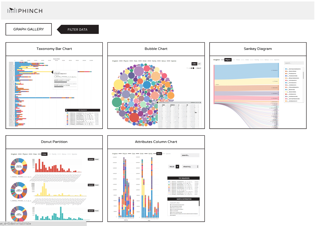
Phinch
Nosotros may now wish to further visualize our results. Nosotros tin can catechumen our shared file to the more widely used biom format and view it in a platform like Phinch.
hands_on Easily-on: Phinch
- Make.biom Tool: toolshed.g2.bx.psu.edu/repos/iuc/mothur_make_biom/mothur_make_biom/one.39.v.0 with the following parameters
- param-collection "shared": the output from Sub.sample tool
- param-collection "constaxonomy": the
taxonomyoutput from Allocate.otu tool- param-file "metadata": the
mouse.dpw.metadatafile you uploaded at the start of this tutorial- View the file in Phinch
- If you expand the the output biom dataset, you will meet a link to view the file at Phinch
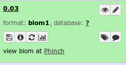
- Click on this link ("view biom at Phinch")
This link volition atomic number 82 you to a Phinch server (hosted by Galaxy), which will automatically load your file, and where y'all can several interactive visualisations:
Determination
Well washed! bays Yous have completed the basics of the Schloss lab's Standard Operating Procedure for Illumina MiSeq information. Yous have worked your manner through the following pipeline:

Key points
16S rRNA gene sequencing analysis results depend on the many algorithms used and their settings
Quality control and cleaning of your data is a crucial footstep in lodge to obtain optimal results
Adding a mock community to serve as a control sample tin can help you asses the error rate of your experimental setup
Nosotros can explore alpha and beta diversities using Krona and Phinch for dynamic visualizations
Often Asked Questions
Have questions nigh this tutorial? Check out the tutorial FAQ page or the FAQ page for the Metagenomics topic to see if your question is listed there. If not, please ask your question on the GTN Gitter Channel or the Galaxy Help Forum
Useful literature
Further information, including links to documentation and original publications, regarding the tools, analysis techniques and the interpretation of results described in this tutorial tin be plant here.
References
- DeSantis, T. Z., P. Hugenholtz, Due north. Larsen, G. Rojas, Due east. L. Brodie et al., 2006 Greengenes, a Chimera-Checked 16S rRNA Gene Database and Workbench Uniform with ARB. Applied and Environmental Microbiology 72: 5069–5072. 10.1128/aem.03006-05
- Liu, Z., T. Z. DeSantis, Chiliad. L. Andersen, and R. Knight, 2008 Accurate taxonomy assignments from 16S rRNA sequences produced by highly parallel pyrosequencers. Nucleic Acids Enquiry 36: e120–e120. 10.1093/nar/gkn491
- Schloss, P. D., Southward. L. Westcott, T. Ryabin, J. R. Hall, Thousand. Hartmann et al., 2009 Introducing mothur: open-source, platform-independent, community-supported software for describing and comparing microbial communities. Appl. Environ. Microbiol. 75: 7537–7541.
- Wooley, J. C., A. Godzik, and I. Friedberg, 2010 A Primer on Metagenomics (P. E. Bourne, Ed.). PLoS Computational Biological science vi: e1000667. ten.1371/journal.pcbi.1000667
- Federhen, Due south., 2011 The NCBI Taxonomy database. Nucleic Acids Research 40: D136–D143. 10.1093/nar/gkr1178
- Bonilla-Rosso, Thou., 50. E. Eguiarte, D. Romero, Grand. Travisano, and V. Souza, 2012 Understanding microbial community multifariousness metrics derived from metagenomes: performance evaluation using faux data sets. FEMS Microbiology Environmental 82: 37–49. 10.1111/j.1574-6941.2012.01405.10
- Quast, C., East. Pruesse, P. Yilmaz, J. Gerken, T. Schweer et al., 2012 The SILVA ribosomal RNA factor database project: improved information processing and web-based tools. Nucleic Acids Research 41: D590–D596. 10.1093/nar/gks1219
- Schloss, P. D., 2012 Secondary construction improves OTU assignments of 16S rRNA gene sequences. The ISME Journal 7: 457–460. x.1038/ismej.2012.102
- Cole, J. R., Q. Wang, J. A. Fish, B. Chai, D. M. McGarrell et al., 2013 Ribosomal Database Projection: data and tools for high throughput rRNA assay. Nucleic Acids Inquiry 42: D633–D642. 10.1093/nar/gkt1244
- Finotello, F., E. Mastrorilli, and B. D. Camillo, 2016 Measuring the diversity of the human being microbiota with targeted side by side-generation sequencing. Briefings in Bioinformatics bbw119. 10.1093/bib/bbw119
- Fouhy, F., A. 1000. Clooney, C. Stanton, M. J. Claesson, and P. D. Cotter, 2016 16S rRNA cistron sequencing of mock microbial populations- impact of DNA extraction method, primer selection and sequencing platform. BMC Microbiology 16: ten.1186/s12866-016-0738-z
- Rognes, T., T. Flouri, B. Nichols, C. Quince, and F. Mahé, 2016 VSEARCH: a versatile open source tool for metagenomics. PeerJ 4: e2584. 10.7717/peerj.2584
- Singer, E., B. Andreopoulos, R. M. Bowers, J. Lee, S. Deshpande et al., 2016 Next generation sequencing data of a defined microbial mock community. Scientific Information 3: 160081. 10.1038/sdata.2016.81
- Balvočiūtė, M., and D. H. Huson, 2017 SILVA, RDP, Greengenes, NCBI and OTT — how practice these taxonomies compare? BMC Genomics xviii: 10.1186/s12864-017-3501-iv
Feedback
Did you employ this fabric every bit an instructor? Experience free to give us feedback on how information technology went.
Did you utilise this fabric as a learner or student? Click the form below to get out feedback.

Citing this Tutorial
- Saskia Hiltemann, Bérénice Batut, Dave Clements, 2019 16S Microbial Analysis with mothur (extended) (Milky way Training Materials). https://training.galaxyproject.org/training-material/topics/metagenomics/tutorials/mothur-miseq-sop/tutorial.html Online; accessed TODAY
- Batut et al., 2018 Community-Driven Data Analysis Training for Biological science Cell Systems 10.1016/j.cels.2018.05.012
details BibTeX
@misc{metagenomics-mothur-miseq-sop, author = "Saskia Hiltemann and Bérénice Batut and Dave Clements", championship = "16S Microbial Analysis with mothur (extended) (Galaxy Training Materials)", year = "2019", calendar month = "05", day = "xx" url = "\url{https://training.galaxyproject.org/grooming-material/topics/metagenomics/tutorials/mothur-miseq-sop/tutorial.html}", note = "[Online; accessed TODAY]" } @commodity{Batut_2018, doi = {10.1016/j.cels.2018.05.012}, url = {https://doi.org/ten.1016%2Fj.cels.2018.05.012}, year = 2018, month = {jun}, publisher = {Elsevier {BV}}, volume = {6}, number = {half-dozen}, pages = {752--758.e1}, author = {B{\'{east}}r{\'{east}}dainty Batut and Saskia Hiltemann and Andrea Bagnacani and Dannon Baker and Vivek Bhardwaj and Clemens Blank and Anthony Bretaudeau and Loraine Brillet-Gu{\'{eastward}}guen and Martin {\v{C}}ech and John Chilton and Dave Clements and Olivia Doppelt-Azeroual and Anika Erxleben and Mallory Ann Freeberg and Simon Gladman and Youri Hoogstrate and Hans-Rudolf Hotz and Torsten Houwaart and Pratik Jagtap and Delphine Larivi{\`{e}}re and Gildas Le Corguill{\'{e}} and Thomas Manke and Fabien Mareuil and Fidel Ram{\'{\i}}rez and Devon Ryan and Florian Christoph Sigloch and Nicola Soranzo and Joachim Wolff and Pavankumar Videm and Markus Wolfien and Aisanjiang Wubuli and Dilmurat Yusuf and James Taylor and Rolf Backofen and Anton Nekrutenko and Björn Grüning}, title = {Community-Driven Data Analysis Training for Biological science}, journal = {Cell Systems} }
Congratulations on successfully completing this tutorial!

How Could I Visualize The Data From Mothur,
Source: https://galaxyproject.github.io/training-material/topics/metagenomics/tutorials/mothur-miseq-sop/tutorial.html
Posted by: simmssestell1948.blogspot.com
0 Response to "How Could I Visualize The Data From Mothur"
Post a Comment