How To Save Data And Plot In One File Matlab

Loading Information into MATLAB for Plotting

In addition to plotting values created with its own commands, MATLAB is very useful for plotting data from other sources, e.g., experimental measurements. Typically this data is bachelor as a apparently text file organized into columns. MATLAB tin can easily handle tab or space-delimited text, merely information technology cannot directly import files stored in the native (binary) format of other applications such as spreadsheets.

The simplest way to import your data into MATLAB is with the load control. Unfortunately, the load command requires that your data file contain no text headings or column labels. To go around this restriction yous must utilise more advanced file I/O commands. Below I demonstrate both approaches with examples. I've included an k-file to handle the more circuitous case of a file with an arbitrary number of lines of text header, in add-on to text labels for each column of data. Though hardly a cure-all, this office is much more flexible than the load command considering it allows you lot to provide documentation inside your data file.

Here'south an outline of this department

The MATLAB load Command
A simple plot of data from a file
Plotting information from files with column headings

The MATLAB `load` Command

In that location is more than ane manner to read data into MATLAB from a file. The simplest, though least flexible, procedure is to utilize the load command to read the entire contents of the file in a unmarried step. The load command requires that the data in the file be organized into a rectangular array. No column titles are permitted. Ane useful course of the load control is

        load name.ext

where ``name.ext'' is the name of the file containing the data. The result of this operation is that the data in ``proper noun.ext'' is stored in the MATLAB matrix variable called name. The ``ext'' string is any 3 grapheme extension, typically ``dat''. Whatever extension except ``mat'' indicates to MATLAB that the data is stored every bit plain ASCII text. A ``mat'' extension is reserved for MATLAB matrix files (see ``assist load'' for more data).

Suppose you had a elementary ASCII file named my_xy.dat that contained two columns of numbers. The following MATLAB statements volition load this data into the matrix ``my_xy'', then copy it into two vectors, 10 and y.

        >> load my_xy.dat;     %  read information into the my_xy matrix 	>> 10 = my_xy(:,1);     %  copy first column of my_xy into x 	>> y = my_xy(:,two);     %  and 2nd column into y

Yous don't need to re-create the data into x and y, of course. Whenever the ``x'' data is needed you could refer to information technology as my_xy(:,1). Copying the data into ``x'' and ``y'' makes the code easier to read, and is more aesthetically highly-seasoned. The duplication of the data will non revenue enhancement MATLAB's memory for most modest data sets.

The load command is demonstrated in the following example.

If the data you wish to load into MATLAB has heading data, e.1000., text labels for the columns, you lot have the following options to deal with the heading text.

Delete the heading information with a text editor and use the load command :-(
Use the fgetl command to read the heading data one line at at time. You lot can then parse the column labels with the strtok control. This technique requires MATLAB version four.2c or after.
Use the fscanf command to read the heading information.

Of these options, using fgetl and strtok is probably the almost robust and user-friendly. If you read the heading text into MATLAB, i.due east., if you don't use the load command, and so you volition have to besides read the plot data with fscanf. The example, Plotting data from files with column headings shows how this is washed.

A simple plot of information from a file

This example show you how to load a simple data ready and plot it.

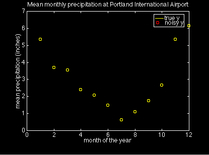
The PDXprecip.dat file contains two columns of numbers. The first is the number of the month, and the 2d is the mean atmospheric precipitation recorded at the Portland International Drome between 1961 and 1990. (For an affluence of weather information like this check out the Oregon Climate Service)

Here are the MATLAB commands to create a symbol plot with the information from PDXprecip.dat. These commands are as well in the script file precipPlot.m for you to download.

        >> load PDXprecip.dat;         %  read data into PDXprecip matrix  	>> month = PDXprecip(:,i);     %  copy first column of PDXprecip into month 	>> precip = PDXprecip(:,two);    %  and second column into precip  	>> plot(calendar month,precip,'o');     %  plot precip vs. month with circles  	>> xlabel('month of the year');           % add axis labels and plot title 	>> ylabel('mean precipitation (inches)'); 	>> title('Mean monthly atmospheric precipitation at Portland International Airport');

Although the data in the month vector is trivial, it is used here anyway for the purpose of exposition. The preceding statments create the following plot.

Plotting data from files with cavalcade headings

If all your data is stored in files that comprise no text labels, the load command is all y'all need. I similar labels, however, because they let me to document and forget almost the contents of a file. To utilise the load for such a file I would take to delete the carefully written comments everytime I wanted to make a plot. Then, in lodge to minimize my effort, I might terminate adding the comments to the data file in the first place. For us command freaks, that leads to an unacceptable increase in entropy of the universe! The solution is to discover a mode to have MATLAB read and deal with the text comments at the top of the file.

The following case presents a MATLAB role that tin read columns of information from a file when the file has an arbitrary length text header and text headings for each columns.

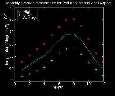
The data in the file PDXtemperature.dat is reproduced below

        Monthly averaged temperature (1961-1990) Portland International Aerodrome 	Source:  Dr. George Taylor, 	Oregon Climate Service, http://world wide web.ocs.oregonstate.edu/ 	 	Temperatures are in degrees Farenheit 	 	Calendar month   Loftier     Low    Average 	1	45.36	33.84	39.half-dozen 	2	l.87	35.98	43.43 	3	56.05	38.55	47.3 	4	sixty.49	41.36	fifty.92 	5	67.17	46.92	57.05 	6	73.82	52.8	63.31 	7	79.72	56.43	68.07 	8	fourscore.fourteen	56.79	68.47 	ix	74.54	51.83	63.18 	x	64.08	44.95	54.52 	xi	52.66	39.54	46.1 	12	45.59	34.75	40.17

The file has a five line header (including blank lines) and each column of numbers has a text label. To use this information with the load control yous would take to delete the text labels and save the file. A improve solution is to accept MATLAB read the file without destroying the labels. Better yet, we should exist able to tell MATLAB to read and utilise the column headings when it creates the plot legend.

At that place is no built-in MATLAB command to read this data, so nosotros accept to write an m-file to do the job. One solution is the file readColData.thousand. The full text of that function won't be reproduced here. You can click on the link to examine the lawmaking and relieve it on your figurer if you like.

Here is the prologue to readColData.m

        part  [labels,x,y] = readColData(fname,ncols,nhead,nlrows) 	%  readColData  reads information from a file containing information in columns 	%               that accept text titles, and possibly other header text 	% 	%  Synopsis: 	%     [labels,10,y] = readColData(fname) 	%     [labels,x,y] = readColData(fname,ncols) 	%     [labels,x,y] = readColData(fname,ncols,nhead) 	%     [labels,x,y] = readColData(fname,ncols,nhead,nlrows) 	%    	%  Input: 	%     fname  = name of the file containing the data (required) 	%     ncols  = number of columns in the data file.  Default = 2.  A value 	%              of ncols is required only if nlrows is also specified. 	%     nhead  = number of lines of header information at the very top of 	%              the file.  Header text is read and discarded.  Default = 0. 	%              A value of nhead is required only if nlrows is also specified. 	%     nlrows = number of rows of labels.  Default = 1 	% 	%  Output: 	%     labels  =  matrix of labels.  Each row of lables is a different 	%                label from the columns of data.  The number of columns 	%                in the labels matrix equals the length of the longest 	%                column heading in the data file.  More than i row of 	%                labels is allowed.  In this case the 2d row of cavalcade 	%                headings begins in row ncol+ane of labels.  The third row 	%                column headings begins in row 2*ncol+1 of labels, etc. 	% 	%          NOTE:  Individual cavalcade headings must non contain blanks 	% 	%     x = column vector of x values 	%     y = matrix of y values.  y has length(x) rows and ncols columns

The first line of the file is the part definition. Following that are several lines of comment statements that form a prologue to the function. Because the kickoff line later on the function definition has a non-blank comment statement, typing ``help readColData'' at the MATLAB prompt volition cause MATLAB to print the prologue in the command window. This is how the on-line help to all MATLAB functions is provided.

The prologue is organized into four sections. First is a brief argument of what the part does. Adjacent is a synopsis of the ways in which the function can be called. Following that the input and output parameters are described.

Here are the MATLAB commands that apply readColData.m to plot the data in PDXtemperature.dat. The commands are also in the script file multicolPlot.1000

        >>  %  read labels and x-y data 	>>  [labels,calendar month,t] = readColData('PDXtemperature.dat',iv,5);  	>>  plot(month,t(:,1),'ro',calendar month,t(:,ii),'c+',calendar month,t(:,3),'1000-');  	>>  xlabel(labels(ane,:));                      % add axis labels and plot championship 	>>  ylabel('temperature (degrees F)'); 	>>  title('Monthly average temperature for Portland International Airport');  	>>  %  add a plot legend using labels read from the file 	>>  legend(labels(2,:),labels(3,:),labels(4,:));

These statments create the following plot.